A sonar example with other than circular and rectangular apertures

Richard Nilsson, Uppsala University, Sweden, has a page for the Thinned Array Sidescan Sonar page. It simulates four 50 kHz circular fishfinder transducers, each with diameter 44 mm and with minimum 60 mm between centers and various ways of combining them into a poor man's sidescan sonar. This has been used as an example here.  

This can be done by starting with a 2D array which is larger than the area covered by the four apertures. The 2D array in this example is set up with one point per mm.

Information about each point in the aperture is stored in the array elem_pts, see the manual for details. An example of an element in this array is

    elem_pts(:,10)' = [ -0.1295,    -0.0205,         0,    1.0000,   10.0000].

These elements are the x, y, and z coordinates of the element followed by the azimuth and elevation element numbers. Ultrasim has a feature which makes it possible for all processing to ignore an element and this is done by setting the azimuth number to a negative value, i.e.

    elem_pts(4,10) = [ -1.0000].

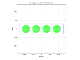
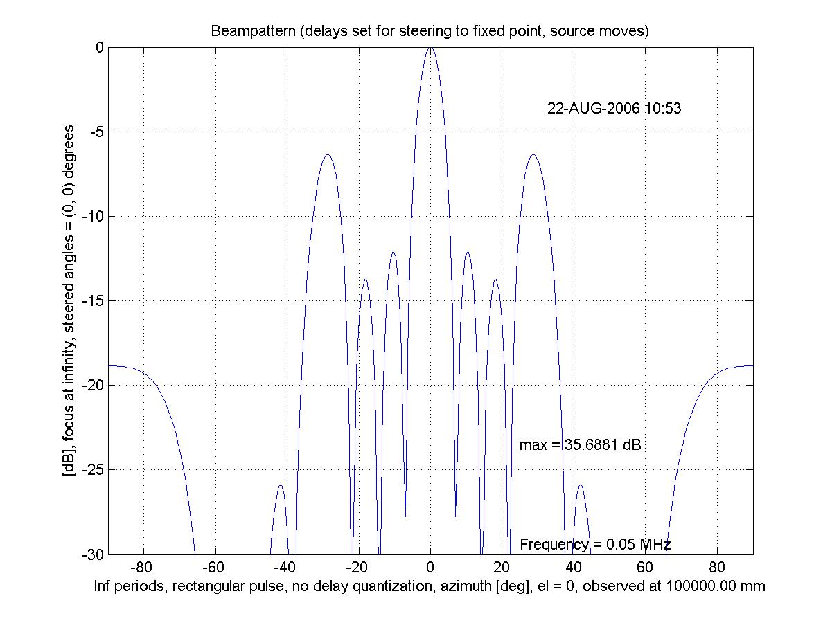
This can be done in a script which is run from the command line. It will thin the full 2D array down to the four circular subapertures above. The code can be found in thin4.html. The resulting beam pattern is shown below. The result is similar to Figs 2a and 2b of Simulation of Sidescan Transducer Arrays.

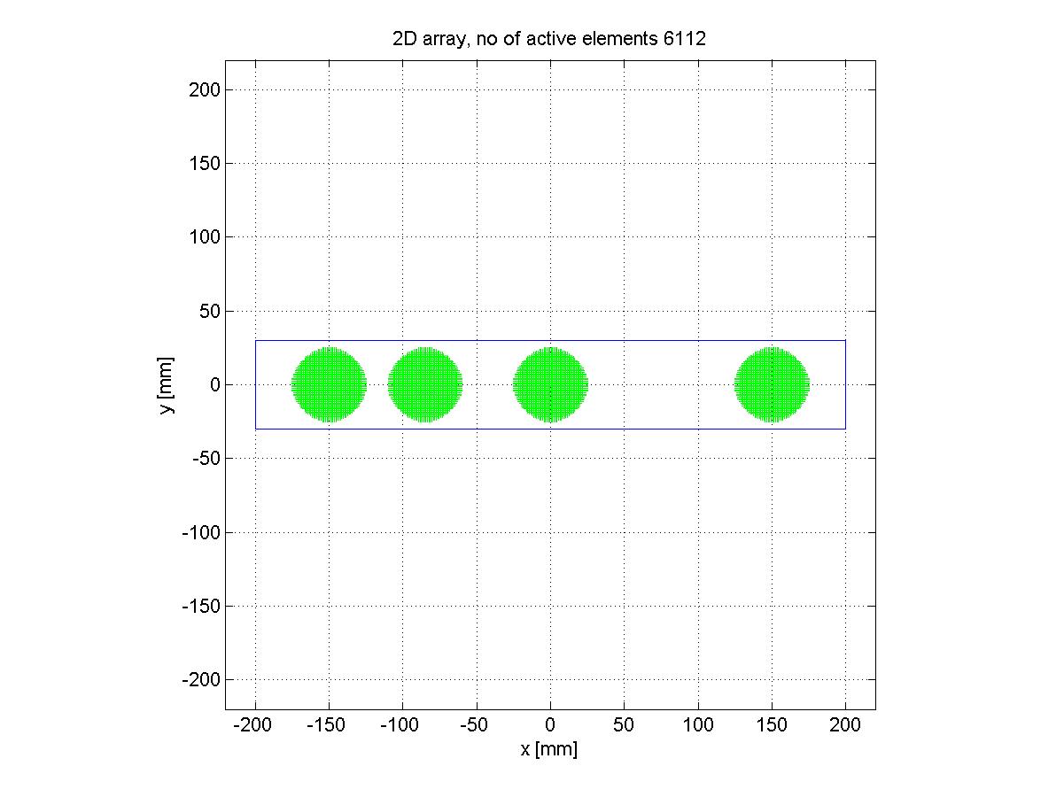
An irregular distribution of the four circular aperture has been proposed in Simulation of Sidescan Transducer Arrays, the second set of Figs 3a and 3b. The code in thin4b.html does that. The aperture is shown below. Notice how the effective aperture is larger than the previous one, but with more 'holes' in the aperture.

The beam pattern is shown here.

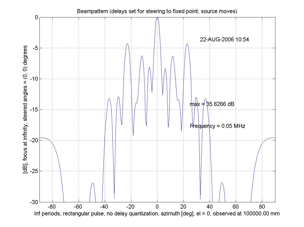
Note that this beam pattern has a narrower mainlobe, but higher side/grating-lobes than before. You gain some and you lose some, unlike in the simulation of Simulation of Sidescan Transducer Arrays which shows the unlikely result of both an improved mainlobe and improved sidelobes.