Ozone Decline over Europe

_{The map displays estimated trend coefficients $\widehat\beta_i$ for summer season ozone, via the generalised additive modelling explained below, for the 302 rural stations, for the period 2000 to 2010. Negative and positive trends are shown using blue and red colours, respectively. The unit is ppb/year. A similar map can be shown for the 210 suburban stations, but here the negative trend is less pronounced, cf. the confidence curves below.}

Ozone

Ozone is a gas that occurs both in the Earth's upper atmosphere and at ground level. Depending on its location in the atmosphere, ozone can be "good" or "bad" for your health and the environment; see the information provided here by the US Environmental Protection Agency. Various measures are taken to limit or phase out the production and use of ozone-depleting substances, in Europe and in other parts of the world. Important in this regard is the Montreal Protocol on Substances that Deplete the Ozone Layer, dating back to 1987, with several later revisions, involving high-level international cooperation. Kofi Annan, Secretary-General of the United Nations, hailed it as having been "perhaps the single most successful international agreement to date".

It ought to be pointed out that the Montreal Protocol mainly relates to the stratospheric layers of ozone, whereas the story we report on here concerns the tropospheric situation, i.e. ozone levels close to ground level.  

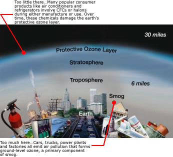
_{Illustration: from the US Environmental Protection Agency.}

The typical mean or median level of summer season ozone at the Airbase rural stations, for the period 2000 to 2010, is around 45-50 ppb, with ppb meaning parts per billion per volume. Such amounts sound almost ridiculously small – think half a small cup of coffee in an enormous water swimming pool of size 10 m x 10m x 10 m. But it matters, and higher amounts may affect your health (and might be particularly bothersome for people with lung and heart diseases), and also disturb plants and crops. These ozone levels also vary substantially, between stations and over time.

Data, model, and analysis

The ozone data utilised for our analyses below stem from the European Environmental Agency’s database Airbase v8, and relate to 302 rural and 210 suburban stations, across Europe. Various meteorological measurements are taken, also from the EURODELTA-Trends project, including daily values of air temperature, relative humidity, wind speed, and so on. At each station, a specially designed generalised additive model has been fitted to the data, using corresponding meteorological data as smooth explanatory variables, including also a day of season variable. Specifically, we have used 

\(\eqalign{ x_1(t)=&\hbox{air temperature at 2 m above ground}, \cr x_2(t)=&\hbox{relative humidity close to surface}, \cr x_3(t)=&\hbox{solar short-wave radiation}, \cr x_4(t)=&\hbox{wind speed at 10 m above ground}, \cr x_5(t)=&\hbox{atmospheric boundary layer height}, \cr x_6(t)=&\hbox{day number relative to 1 May}. \cr}\)

Crucially, we include in our models also a linear long-term trend, describing the potential change in ozone over time. Thus, at each station, the model is

\(O_3(t)=\alpha+\beta t+\sum_{j=1}^6 s_j(x_j(t))+\varepsilon(t),\)

relating the daily ozone values $O_3(t)$ to smooth functions $s_j(x_j(t))$ of the meteorological and day of season variables and to the looked-for linear trend $\alpha+\beta t$ in ozone, where $t$ represents time in years, from 2000; finally, $\varepsilon(t)$ represents the error term, taken normally distributed with mean zero.The linear trend may be interpreted as a meteorologically adjusted trend at each station, mainly influenced by trends in various precursors to ozone from emissions of nitrogen oxides (NOx) and volatile organic compounds (VOCs) from traffic and industry.

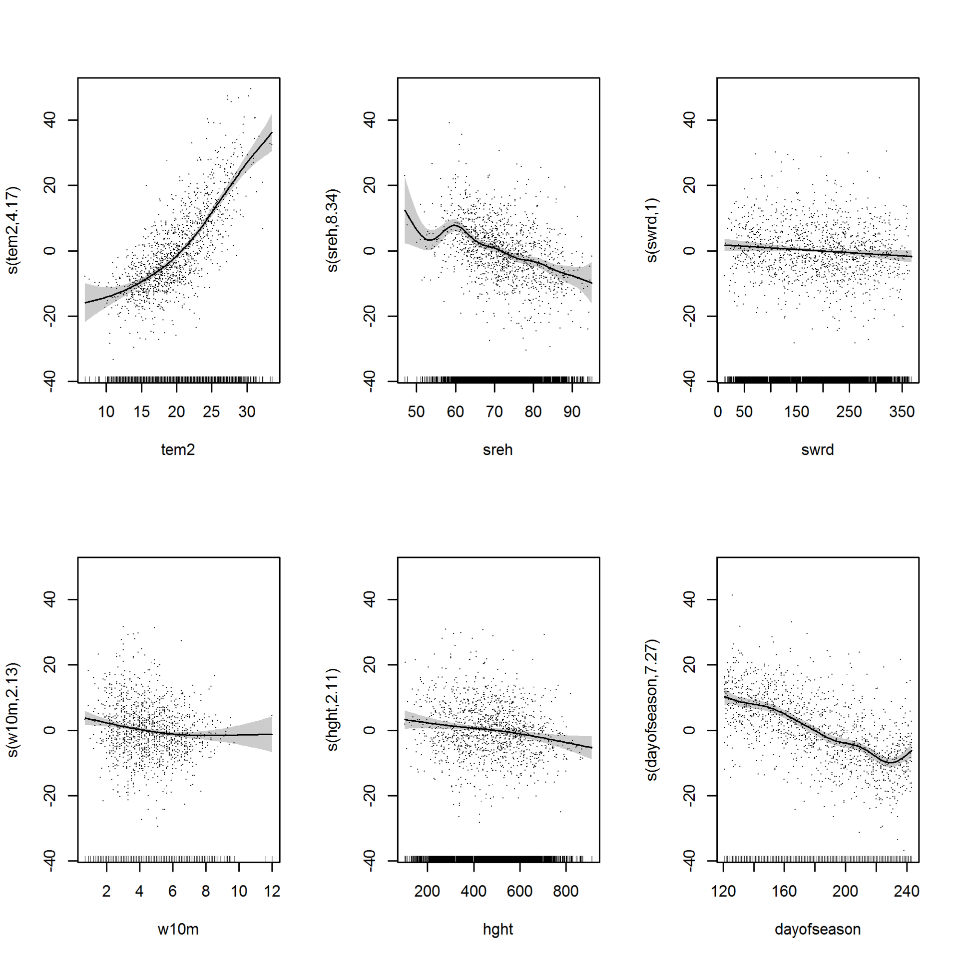
The point of the generalised additive modelling apparatus is that the $s_j(x_j)$ functions, used in the $O_3(t)$ modelling equation above, need not be linear or indeed given parametric functions, but are allowed to enter the model as smooth nonparametric curves. The figure above indicates these estimated $s_j(x_j)$ functions, along with error bands and residuals. We learn e.g. that the ozone level depends on $x_2(t)$ in a rather nonlinear fashion, and that the solar radiation $x_3(t)$ does not appear to affect the ozone level very much. 

Our focus here is on the trend over time, specifically the $\beta$ parameter. Like the ozone median level itself, also the trend parameter varies across Europe. Analysing the model above yields an estimate $\widehat\beta_i$, for station $i$, along with an estimated standard deviation $\sigma_i$. As seen from the ozone map above, a negative (downward) trend is found at most of the rural stations, with the strongest declines at some of the Italian sites. Some of the UK sites, however, show increasing levels of ozone.

The grander question is whether the overall European tropospheric ozone trend has been negative, for the 2000 to 2010 decade. We answer this by modelling the individual $\beta_i$ as coming from an appropriate background distribution, a normal ${\rm N}(\beta_0,\tau^2)$. Using modern meta-analysis, via confidence distributions, as developed in Schweder and Hjort (2016, Ch. 13), we can estimate both the overall trend parameter $\beta_0$ and the spread parameter $\tau$, along with confidence curves, say ${{\rm cc}}(\beta_0)$ and ${{\rm cc}}(\tau)$. These are displayed below. The precision parameters $\sigma_i$, related to how precise the individual $\widehat\beta_i$ estimates are, are involved in these methods.

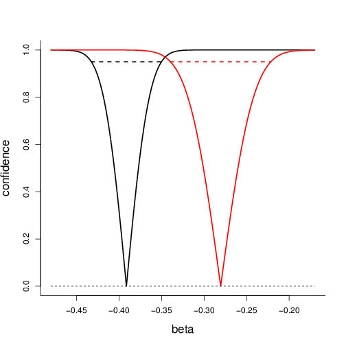
_{Confidence curves for the overall trend coefficient $\beta_0$ of the summer season ozone in Europe, at the rural (black, left) and suburban stations (red, right), for the period 2000 to 2010 (left plot). The unit is again in ppb/year.}

As seen in the figure here, the confidence curve to the left points to an overall average decline in summer season ozone in rural Europe of -0.391 ppb per year, or -3.91 ppb per decade, with [-4.33, -3.50] as a 95 percent confidence interval for the latter. For the suburban stations, the overall estimate is -0.281 ppb per year, or -2.81 per decade, with 95 percent interval [-3.40,-2.22]. This represents a small but significant decline in the ozone levels corresponding to around 0.8 percent per year, or 8 percent per decade. The decline for the suburban stations is about 6 percent per decade.

Since the individual generalised additive model based trends at the stations were meteorologically adjusted, this decline is probably for the most part due to a reduction in emissions of precursors to ozone such as NOx and VOCs from traffic and industry. This is good news!

It is also of interest to assess the degree of variation, for this negative ozone trend parameter, across Europe, i.e. the spread parameter in the $\beta_i\sim{{\rm N}}(\beta_0,\tau^2)$ distribution. Via confidence analysis, as per Schweder and Hjort (op. cit.), we find median confidence estimates 0.36 and 0.43 for $\tau$, for the rural and suburban stations, and with 95 percent intervals [0.33, 0.39] and [0.39, 0.48], respectively. In particular, the rural terrain, with the strongest decline, is also associated with smaller variation in this decline parameter. This information (and more) is summarised in the two confidence curves shown here, for the rural spread $\tau_r$ and the suburban spread $\tau_s$.

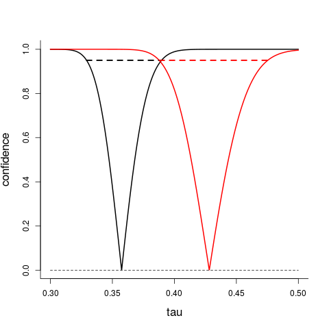
_{Confidence curves ${{\rm cc}}(\tau_r)$ (left, black) and ${{\rm cc}}(\tau_s)$ (right, red) for the rural and suburban spread parameters.}

Concluding remarks 

1. Autocorrelation. In the analysis reported on above potential autocorrelation in the residuals is not taken into account. However, certain tests with generalised additive modelling, where this was taken into account, gave only small changes in the estimated trend values. A similar remark applies to the possibility of allowing the residual $\varepsilon_i(t)$ terms in our generalised additive model have variances which also depend on the covariates $x_j(t)$.  

2. Spatial correlation. The meta-analyses we report on above, leading to confidence curves for overall negative trend parameter $\beta_0$ and spread parameter $\tau$, have used the assumption that the meteorological stations are far enough away from each other to make their underlying $\beta_i$ parameters approximately independent. More refined analyses are possible, taking spatial correlation into account. 

3. Other models. Other statistical models can also be considered, analysed, and assessed here, for how the meteorological covariates $x_j(t)$ affect the ozone levels, using e.g. parametric forms for the $s_j(x_j)$ terms. This would also involve development of model selection tools for additive models. 

4. After 2011. Our story relates specifically to the decade from 2000 to 2010. There are international data-gathering programmes at work also for what is happening after 2011, and EEA (the European Environment Agency) and NILU (the Norwegian Institute for Air Research) are involved both in the experimental design and in the ensuing statistical analyses. It will certainly be of interest to compare the story we have told here with similar data for the 2011 to 2020 decade. 

5. The Ozone Hole. There is also an interesting statistical story around the somewhat slow scientific detection of the famous Ozone Hole, related to how NASA scientists interpreted their data. For some years they tended to indirectly classify genuine measurements as "outliers". A better statistical understanding, also of so-called robust methods, would perhaps have helped them to find the hole (i.e. the decline in stratospheric ozone) earlier.

6. The UN GEO-6 Report. According to the United Nations GEO-6 report, released in Nairobi, March 2019, as many as six million people die prematurely, each year, due to air pollution. So statisticians should be on board, helping to identify the more dire factors contributing to the bleak current state of affairs, so that preventive measures perhaps can be taken. In this connection, you may wish to browse through the breathelife2030 site, check conditions in the city you live in, and perhaps contemplate the number of air pollution related premature deaths in your country. 

7. Declining trends & declining trends. Also the non-statisticians of the world learn about spurious correlations, phenomena of no apparent relation that somehow nevertheless demonstrate high correlation over time (divorce rates in Maine have developed extremely similarly to the U.S. per capita consumption of margarine; a nation's chocolate consumption correlates beautifully with its number of Nobel Prize winners;  etc. etc.). We may report one curious statistical and indeed FocuStat project related incident in this regard. The present blog story is about a certain overall trend, that of ozone levels, being in decline over the 2000-2010 decade, complete with delicate analysis of the pertinent $\beta_0$ parameter. As such the story curiously correlates with another FocuStat study, concerning the slimming of the Antarctic minke whales, over the 1988-2005 time period. Again, delicate analysis of complex data is necessary to uncover a decline-over-decades parameter $\beta_0$, along with controversies and conflicting evidence and even politics entering the soup; see Cunen and Hjort (2018). So perhaps there's a causal connection between the European ozone levels and the declining energy storage for minke whales near the South Pole. Tilfeldig? Neppe.

References

Cunen, C. (2019). Confidence curves for dummies. In FocuStat Summary Report, page 5.

Cunen, C. and Hjort, N.L. (2018). Whales, Politics, and Statisticians. FocuStat blog post.

European Environment Agency (2018). EEA Airbase - The European Air Quality Database, Version 8.

Pukelsheim, F. (1990). Robustness of statistical gossip and the Antarctic ozone hole. Institute of Mathematical Statistics Bulletin.

Schweder, T. and Hjort, N.L. (2016). Confidence, Likelihood, Probability: Statistical Inference With Confidence Distributions. Cambridge University Press, Cambridge.

Solberg, S., Walker, S.-E., Schneider, P., Guerreiro, C., Colette, A. (2018). Discounting the effect of meteorology on trends in surface ozone: Development of statistical tools. ETC/ACM Technical Paper 2017/5.

Wood, S.N. (2017). Generalized Additive Models: An Introduction with R (2nd edition). Chapman and Hall/CRC Press.